Exercise Sheet
Choose PDF for printing or Word for editing.
Introduction to Statistics · Topic 3
Topics 1 and 2 prepared two sides of the same problem. Topic 1 showed how to describe the sample in front of us. Topic 2 showed that a statistic, such as a sample mean, changes when a new random sample is drawn. We are now ready to put those ideas together and ask what an observed sample can tell us about a larger population.
Imagine that a sample has a mean planning score of 54 when a reference value is 50. The four-point difference is easy to calculate, but it raises a more interesting question: is the sample revealing a population difference, or could ordinary sample-to-sample variation have produced a difference this large? That variation is not an inconvenience to hide. It is the information that lets us judge how much uncertainty surrounds the result.
Statistical inference is the process of using a sample to reason carefully about a population. An inference does not turn a sample result into certainty. It combines the result with a probability model, the study design, and explicit assumptions.
This topic develops two closely related tools for keeping that uncertainty visible. A confidence interval gives a range of parameter values compatible with the estimate and its uncertainty. A hypothesis test asks whether the sample result would be unusually far from a stated population value under a specified model. Both tools depend on the sampling distributions introduced in Topic 2, and both help us move from describing one sample toward making a careful, limited population conclusion.
Guiding question: How can one sample teach us something about a population while keeping uncertainty honest?
Inference is not a leap from one sample to a guaranteed truth. It is a structured argument whose uncertainty remains visible.
By the end of this topic, you should be able to:
A population is the full group about which a question is asked. A parameter is a numerical property of that population, such as its mean \(\mu\). Parameters are usually unknown.
A sample is the observed subset. A statistic is a number calculated from the sample, such as the sample mean \(\bar{x}\). An estimator is the rule used to calculate a statistic for the purpose of estimating a parameter. For example, the sample mean is an estimator of the population mean.
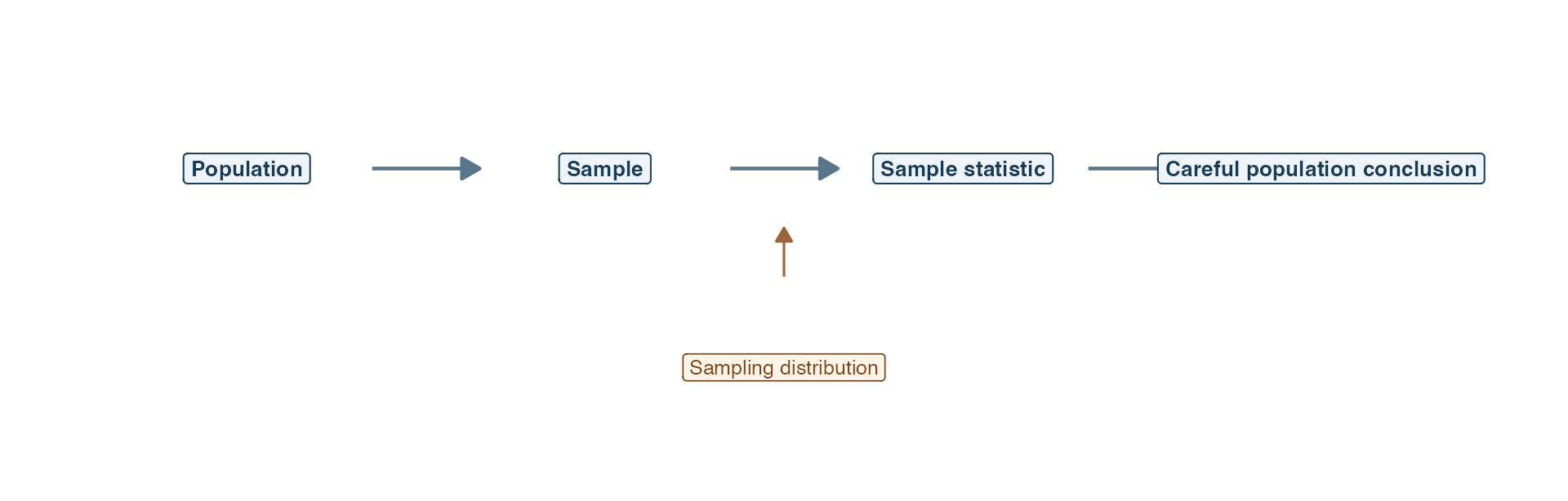
Follow the top row from left to right. The population is the group we ultimately want to understand, but we observe only a sample. That sample produces a statistic, and the statistic supports a cautious conclusion about the population. The sampling distribution appears underneath because it supplies the missing link: it tells us how the statistic would vary if the sampling process were repeated. Without that variation, the jump from one sample number back to a population claim would have no measure of uncertainty.
| Object | Example for a mean | What it describes |
|---|---|---|
| Population parameter | \(\mu\) | The unknown population mean |
| Sample statistic | \(\bar{x}\) | The mean calculated from the observed sample |
| Standard deviation | \(s\) | Variation among individual observed values |
| Estimated standard error | \(s/\sqrt{n}\) | Estimated variation among sample means across repeated samples |
The standard error is the bridge in the figure. It tells us how much an estimator would ordinarily vary across repeated random samples under the model. We first use that information to build an interval around an estimate.
A point estimate is one numerical estimate of a parameter. For example, \(\bar{x}=52\) is a point estimate of \(\mu\). One number alone does not show how precise it is.
A confidence interval adds lower and upper limits around the point estimate. Its confidence level describes the long-run success rate of the interval-producing method. A 95% confidence procedure is designed so that, across many repetitions of the same sampling process, about 95% of the calculated intervals cover the fixed population parameter and about 5% miss it.
Most confidence intervals introduced here follow one simple structure:
\[ \text{point estimate} \ \pm\ \text{critical value}\times\text{standard error}. \]
The point estimate places the center of the interval. The critical value determines how many standard errors the method extends on either side, and the standard error carries information about sampling uncertainty. The product of the critical value and standard error is called the margin of error. You do not need to memorize every interval formula at once. First learn to recognize these three pieces and what each contributes.
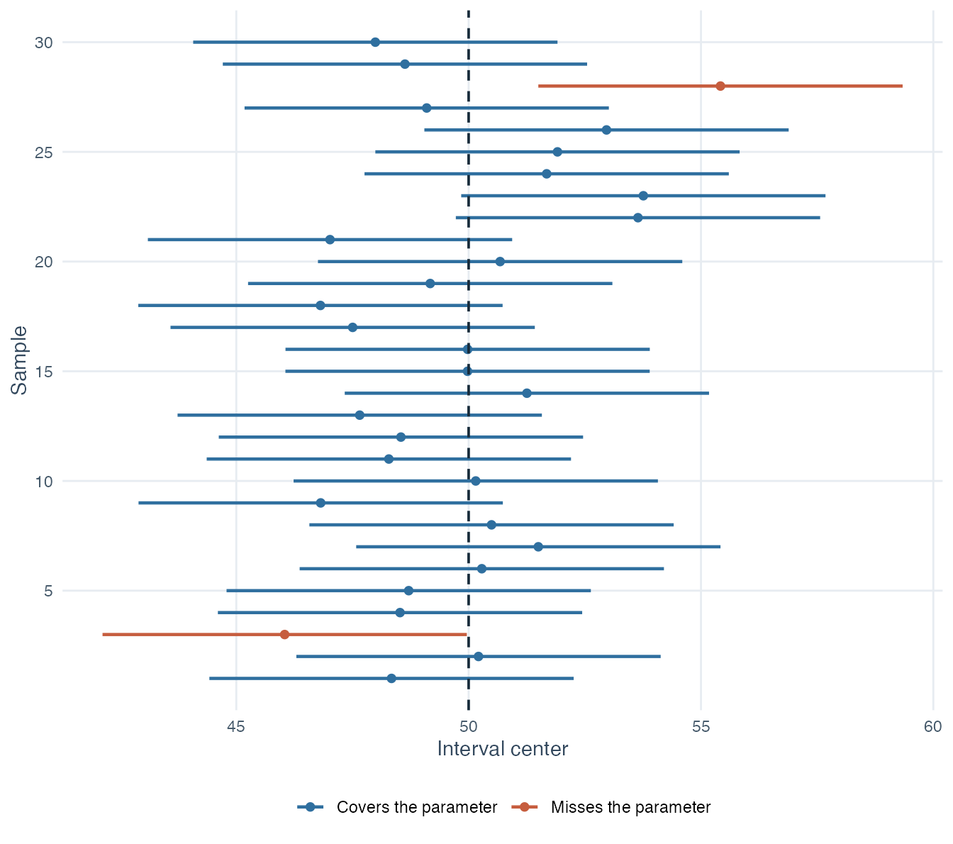
Read the figure one horizontal row at a time. Each dot is the mean from a different sample, and each horizontal segment is the confidence interval built around that sample mean. The vertical line marks the one population mean that all samples are trying to estimate. Blue intervals cross that fixed line and therefore cover the parameter, whereas orange intervals miss it. The figure shows 30 repetitions, so it is only an illustration of the long-run idea. A 95% procedure is not required to cover exactly 95% in every small batch of samples.
Once one interval has been calculated, its endpoints are fixed and the parameter is fixed. We therefore do not say that the parameter now has a 95% probability of lying inside that completed interval. The 95% describes the procedure across repetitions.
Three ingredients control interval width:
A narrow interval describes greater precision under the sampling model. It does not repair biased measurement, selective sampling, or a poor study design.
The same sampling model can also be used to examine a specific proposed value. That is the role of a hypothesis test.
A statistical hypothesis is a statement about a population parameter. Two statements are considered together:
Suppose \(\mu_0\) is a reference population mean and \(\mu\) is the population mean under study. The form of \(H_1\) determines which sample results count as evidence against \(H_0\).
| Research question | Null hypothesis | Alternative hypothesis | Test direction |
|---|---|---|---|
| Is the mean larger? | \(H_0:\mu=\mu_0\) | \(H_1:\mu>\mu_0\) | Upper tailed |
| Is the mean smaller? | \(H_0:\mu=\mu_0\) | \(H_1:\mu<\mu_0\) | Lower tailed |
| Is the mean different? | \(H_0:\mu=\mu_0\) | \(H_1:\mu\ne\mu_0\) | Two sided |
A tail is an end of a probability distribution. The significance level, written \(\alpha\) (alpha), is the total probability assigned to results that the decision rule will treat as sufficiently incompatible with \(H_0\) when \(H_0\) is true. Here, \(\alpha=0.05\) is commonly used. An upper-tailed test places the rejection region in the high end, a lower-tailed test uses the low end, and a two-sided test divides the chosen significance level between both ends. The next section explains why \(\alpha\) is also the long-run probability of a Type I error.
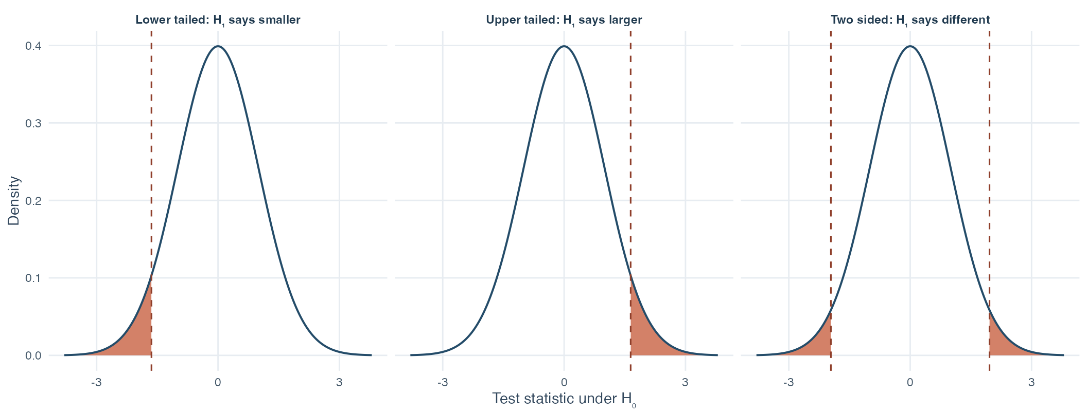
The three panels use the same total significance level but place it differently. In the lower-tailed panel, only unusually small statistics count against \(H_0\). In the upper-tailed panel, only unusually large statistics count. In the two-sided panel, unusual results in either direction count, so half of \(\alpha\) appears in each tail. The unshaded center contains results for which the rule fails to reject \(H_0\). It does not represent proof that \(H_0\) is correct.
The direction must be justified by the research question and fixed before the data are examined. Choosing a one-sided test after seeing the direction of the sample result would invalidate the chosen significance level.
A hypothesis test uses a sample to choose between two actions: reject \(H_0\), or fail to reject \(H_0\). Failing to reject means that the sample did not provide sufficiently unusual evidence under the chosen rule. It does not prove that \(H_0\) is true.
Because the decision is based on a sample, it can be wrong:
| What is true in the population | Fail to reject \(H_0\) | Reject \(H_0\) |
|---|---|---|
| \(H_0\) is true | Correct non-rejection | Type I error |
| The specified \(H_1\) is true | Type II error | Correct rejection |
Read the rows as the unknown population reality and the columns as the action taken from the sample. If \(H_0\) is true, rejection creates a Type I error. If the specified alternative is true, failure to reject creates a Type II error. The two diagonal cells are correct decisions. Under a specified alternative, the long-run probability of the correct rejection in the lower-right cell is called power.
A Type I error occurs when the procedure rejects \(H_0\) even though \(H_0\) is true. Its long-run probability is the significance level \(\alpha\) introduced above.
A Type II error occurs when the procedure fails to reject \(H_0\) even though the specified alternative is true. Its probability is written \(\beta\) (beta). The consequences of the two errors depend on the research setting. Neither error is automatically the more acceptable one.
Consider a study of a genuinely helpful teaching program. A Type I error would recommend the program even though it does not improve the population mean, potentially spending time and resources without a benefit. A Type II error would miss a real improvement and leave the existing program unchanged. These consequences show why error probabilities help determine how cautious the testing rule should be and how much data a study needs.
The significance level is chosen before inspecting the result. It is a property of the procedure under its assumptions, not the probability that this particular decision is wrong.
A test statistic is a standardized number calculated from the sample. It compares the observed difference with the amount of sampling variation expected under \(H_0\). A general pattern is
\[ \text{test statistic} = \frac{\text{observed estimate}-\text{value stated by }H_0} {\text{standard error of the estimate}}. \]
The numerator is the observed distance from the null value in the variable’s original units. The denominator is the amount by which the estimate ordinarily varies across repeated samples under the model. Dividing one by the other answers a plain question: how many standard errors away from the null value is this estimate?
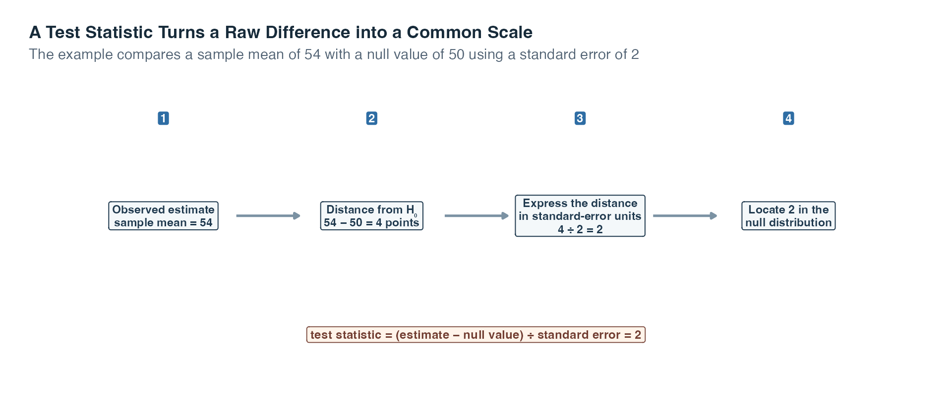
Read the boxes from left to right. The first box contains the observed estimate. The second subtracts the value proposed by \(H_0\), so the raw distance is 4 points. The third divides that distance by the standard error of 2, giving a test statistic of 2. The final box reminds us that the number becomes evidence only after it is located in the correct null distribution.
The diagram connects the formula to its meaning: a statistic of 2 says that the estimate lies two standard errors from the null value. It does not say that the effect equals 2 points, because the original four-point distance and the standardized value answer different questions. It also does not provide a p-value by itself. The null distribution, the direction of \(H_1\), and the prespecified significance level still determine which values count as sufficiently unusual.
The null distribution is the probability distribution of the test statistic when \(H_0\) and the model assumptions hold. It tells us which values are ordinary and which are unusual under the reference statement.
After choosing \(\alpha\), the rejection region contains test-statistic values that lead to rejection of \(H_0\). A critical value is a boundary of that region. The logic follows the same order every time:
A result is called statistically significant at level \(\alpha\) when the procedure rejects \(H_0\). This phrase refers to the testing rule. It does not state that the effect is large or important.
A p-value is the probability, calculated under \(H_0\), of obtaining the observed test statistic or one more extreme in the direction defined by \(H_1\). For a two-sided test, equally extreme values in both directions count.
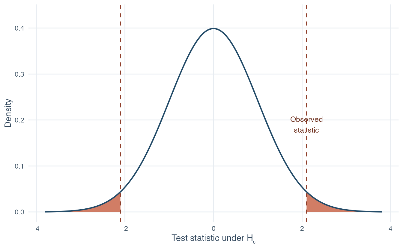
The curve shows test-statistic values expected under \(H_0\). Zero is at the center because this standardized null model expects no departure from the null value. The observed statistic is \(2.10\), and a two-sided question treats \(-2.10\) as equally far from zero. The two shaded tails therefore include every result at least as extreme as the observed result in either direction. Their combined area is the p-value.
For the illustrated standard-normal statistic \(z=2.10\), the two-sided p-value is
\[P(Z\leq-2.10)+P(Z\geq2.10)\approx0.036.\]
The p-value and critical-value approaches give the same decision when they use the same model, direction, and \(\alpha\):
A p-value is not the probability that \(H_0\) is true. It is not the probability that chance caused the result. It also does not measure effect size or practical importance.
The p-value answers an evidence question under \(H_0\). The next section asks a different question: how large and substantively meaningful is the effect?
An effect size describes the size of a difference or relationship, separately from its statistical significance. For a one-sample mean question with known population standard deviation \(\sigma\), we use the standardized effect
\[ \delta=\frac{\mu-\mu_0}{\sigma}. \]
The numerator is the population difference of interest. Dividing by \(\sigma\) expresses that difference in population standard-deviation units. The sign gives direction, while \(|\delta|\) gives magnitude.
Power is the probability that a test rejects \(H_0\) when one specified alternative value is true:
\[\text{Power}=1-\beta.\]
Power is not one fixed property of a study. It changes with the alternative effect being considered. Holding the other ingredients constant:
| Change | Effect on power | Reason |
|---|---|---|
| Increase sample size \(n\) | Increases | The standard error becomes smaller |
| Increase effect magnitude \(|\delta|\) | Increases | The alternative lies farther from \(H_0\) |
| Lower \(\alpha\) | Decreases | The rejection boundary becomes harder to cross |
| Use a justified one-sided rather than two-sided test | Increases in the chosen direction | All of \(\alpha\) is placed in one tail |
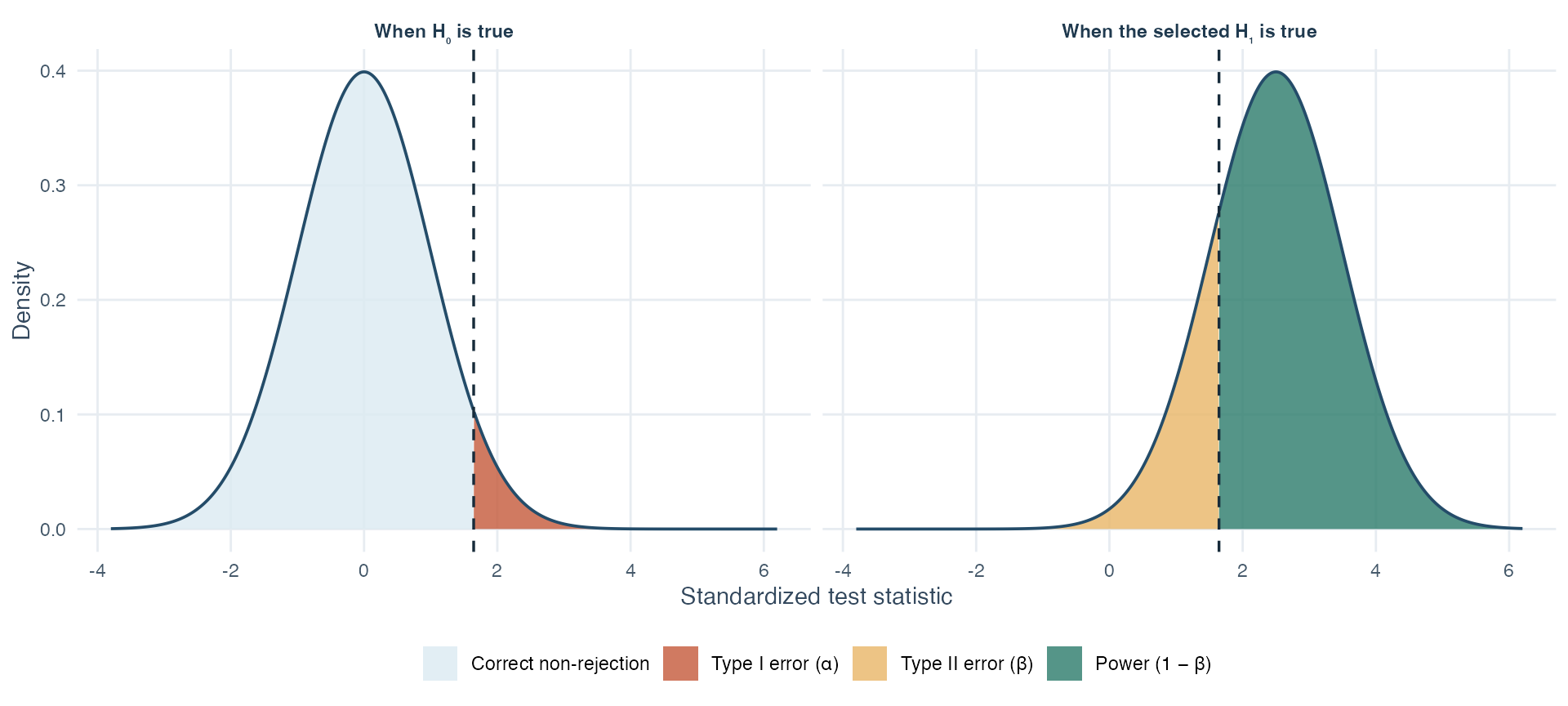
The figure holds the critical boundary fixed. Under \(H_0\), crossing it is a Type I error. Under the specified \(H_1\), crossing it is a correct detection. Moving the alternative distribution farther away or narrowing both distributions through a larger sample increases the power area.
For the one-sided z planning model used here, the required sample size can be written as
\[ n = \left( \frac{z_{1-\alpha}+z_{1-\beta}}{\delta} \right)^2. \]
Here \(z_{1-\alpha}\) sets the rejection boundary, \(z_{1-\beta}\) represents the desired power because power is \(1-\beta\), and \(\delta\) is the standardized effect the study is meant to detect. The result is always rounded up to the next whole observation. This formula is a planning tool for the stated model, not a universal sample-size rule for every statistical procedure.
Power planning should happen before data collection. Researchers first state the smallest difference that would matter in practice, then determine the sample size needed to detect that difference with a chosen power. Calculating power only for the effect already observed in the same data does not answer that planning question.
A statistically significant result says that the observed statistic crossed the predeclared evidence threshold under \(H_0\). It does not say that the difference is large enough to matter.
With a very large sample, a small effect can be estimated precisely and become statistically significant. With a small sample, an important effect can remain undetected because the standard error is large and power is low. A responsible report therefore gives the estimated effect, a confidence interval, and the study context alongside the p-value.
Ask two separate questions: “Is the result difficult to reconcile with \(H_0\) under this model?” and “Is the estimated difference large enough to matter in this setting?”
We now turn from the general logic to the distributions used for tests and intervals about means.
A one-sample procedure compares one sample mean with a reference value \(\mu_0\).
If the population standard deviation \(\sigma\) is known and the stated normal model applies, the z statistic is
\[ z=\frac{\bar{x}-\mu_0}{\sigma/\sqrt{n}}. \]
In most applications \(\sigma\) is unknown. Replacing it with the sample standard deviation \(s\) gives
\[ t=\frac{\bar{x}-\mu_0}{s/\sqrt{n}}. \]
Under \(H_0\) and the model assumptions, this statistic follows a t distribution. A t distribution is a symmetric reference distribution shaped much like the standard normal distribution, but with heavier tails. Heavier tails mean that more probability is assigned to values far from zero because estimating \(\sigma\) adds uncertainty.
The exact t distribution is identified by its degrees of freedom, abbreviated \(df\). Degrees of freedom describe how much independent information remains after estimating required quantities. For the one-sample t procedure,
\[df=n-1.\]
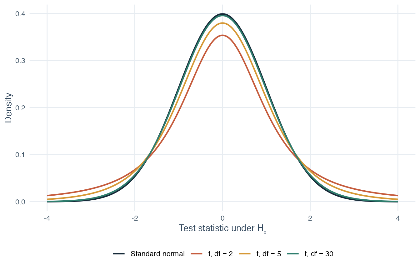
All four curves are centered at zero. The curves with 2 and 5 degrees of freedom place visibly more area in the tails, reflecting the extra uncertainty from estimating the population standard deviation with little data. By 30 degrees of freedom, the t curve is close to the normal curve, although the correct t reference still uses its actual degrees of freedom.
The t and standard-normal shapes become more similar as the sample grows. This is a gradual change, not a universal rule that every study becomes valid at one sample-size cutoff.
For a two-sided interval with unknown \(\sigma\), the matching t-based confidence interval is
\[ \bar{x}\ \pm\ t_{1-\alpha/2,\;n-1}\frac{s}{\sqrt{n}}. \]
Here \(t_{1-\alpha/2,\;n-1}\) is the critical t value with cumulative probability \(1-\alpha/2\) and \(n-1\) degrees of freedom. The quantity multiplied by the critical value is the estimated standard error.
For a two-sided test of \(H_0:\mu=\mu_0\) at level \(\alpha\), the test and the matching \((1-\alpha)\) confidence interval agree:
This agreement requires the same model, assumptions, confidence level, and two-sided alternative.
The formula depends on how observations are connected. The number of columns in a dataset is not enough to decide. We must identify who or what produced each value.
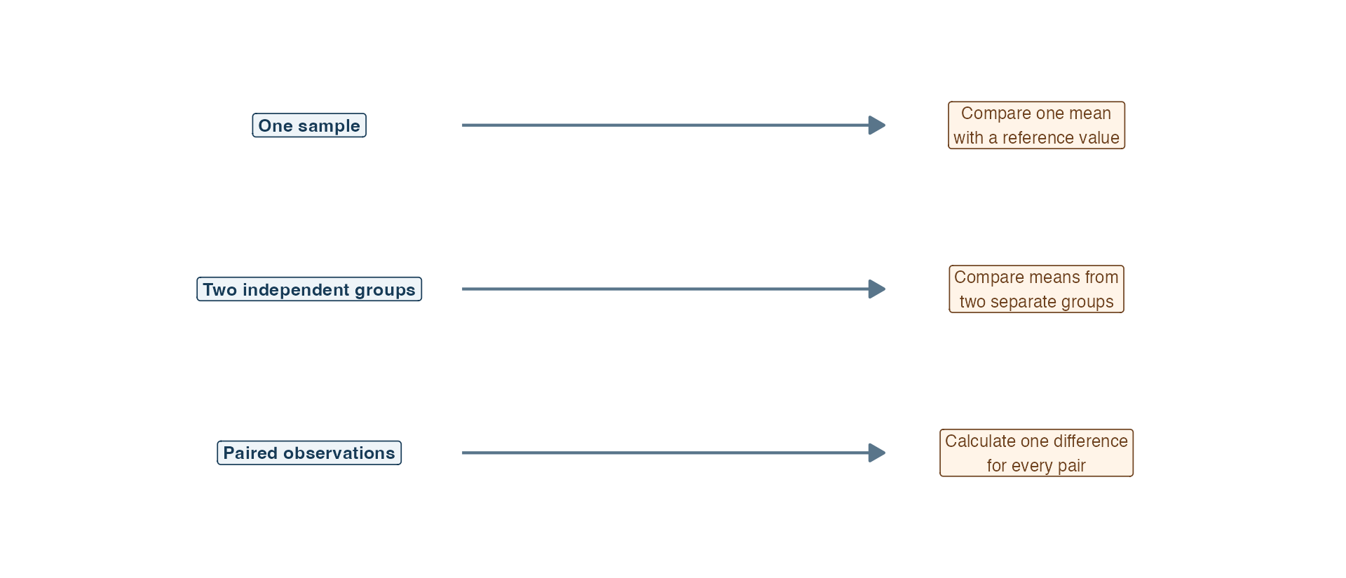
The top row of the figure has one sample and one fixed reference value. The middle row has two separate groups, so no value in one group is linked to a particular value in the other. The bottom row begins with linked measurements and turns each link into one difference score. This is the decision to make before selecting a formula.
| Design | Data structure | Quantity tested |
|---|---|---|
| One sample | One value per sampled unit | \(\mu-\mu_0\) |
| Two independent samples | Each unit belongs to only one group | \(\mu_1-\mu_2\) |
| Paired samples | Two linked values belong to the same person or matched pair | Mean difference \(\mu_d\) |
The final column identifies the population quantity behind each test. A one-sample procedure concerns one mean minus a reference value. An independent-samples procedure concerns a difference between two population means. A paired procedure concerns the population mean of within-pair differences. Similar-looking data can therefore lead to different questions and different standard errors.
An observation is independent when its value is not paired with or determined by another observation in the analysis. Paired observations are deliberately linked, such as a before and after score from the same person. Treating paired values as independent discards the connection that the design created.
For two independent groups, let \(\bar{x}_1\) and \(\bar{x}_2\) be the sample means, \(s_1^2\) and \(s_2^2\) the sample variances, and \(n_1\) and \(n_2\) the sample sizes. The pooled procedure taught here assumes equal population variances and combines the two sample variances into a pooled variance:
\[ s_p^2= \frac{(n_1-1)s_1^2+(n_2-1)s_2^2} {n_1+n_2-2}. \]
Pooling combines the two sample variance estimates under the equal-variance model. The standard error of the mean difference is
\[ SE(\bar{x}_1-\bar{x}_2) = s_p\sqrt{\frac{1}{n_1}+\frac{1}{n_2}}, \]
and the test statistic is
\[ t= \frac{\bar{x}_1-\bar{x}_2} {s_p\sqrt{1/n_1+1/n_2}}, \qquad df=n_1+n_2-2. \]
The matching two-sided confidence interval for the population mean difference is
\[ (\bar{x}_1-\bar{x}_2) \ \pm\ t_{1-\alpha/2,\;n_1+n_2-2} s_p\sqrt{\frac{1}{n_1}+\frac{1}{n_2}}. \]
The interval uses the same pooled standard error and equal-variance model as the test. If it excludes zero, the matching two-sided test rejects a zero population mean difference.
The calculation is easier to follow as a four-part recipe. First, summarize each group separately. Second, combine their two variance estimates into \(s_p^2\) under the equal-variance assumption. Third, use \(s_p\) and both sample sizes to estimate the standard error of the mean difference. Fourth, divide the observed difference by that standard error. The numerator tells us how far apart the groups are. The denominator shows how much that difference would ordinarily vary from sample to sample under the model.
This model requires independent observations, equal population variances, and normally distributed values within each population for exact small-sample inference. With sufficiently large samples, the procedure can be less sensitive to nonnormality, but sample size does not repair dependence, biased sampling, or a badly chosen outcome.
Many software packages use a different independent-samples procedure by default. This topic follows the pooled equal-variance procedure introduced here. The reported name and calculation must agree.
Random assignment means using a chance process to determine which experimental condition each participant receives. In a well-run experiment, it can support a causal comparison because the assignment process aims to prevent the groups from differing systematically before the intervention. A significant difference between preexisting groups in an observational study does not by itself show that group membership caused the difference.
For paired data, first define one difference score for every pair:
\[d_i=x_{i,\text{after}}-x_{i,\text{before}}.\]
The order must be stated because reversing it reverses every sign. Once the differences have been calculated, the problem becomes a one-sample t procedure for \(H_0:\mu_d=0\):
\[ t=\frac{\bar{d}}{s_d/\sqrt{n}}, \qquad df=n-1. \]
Here \(n\) is the number of complete pairs, \(\bar{d}\) is their mean difference, and \(s_d\) is the standard deviation of the difference scores. The relevant normality condition concerns the distribution of the differences, not each measurement considered separately.
The matching two-sided confidence interval is
\[ \bar d \ \pm\ t_{1-\alpha/2,\;n-1}\frac{s_d}{\sqrt n}. \]
This interval estimates the population mean of the declared difference, so its sign changes if the subtraction order is reversed.
The paired procedure is also appropriate for intentionally matched units, such as matched cases and controls, when each match defines a meaningful pair.
The z and t procedures are parametric procedures, meaning that their null distributions are derived using specified population parameters and distributional conditions. This topic also introduces rank-based procedures as alternatives when the original-value distribution does not suit the corresponding parametric model.
A rank is the position of a value after all relevant values are sorted from smallest to largest. Replacing measurements with ranks preserves their order but discards the exact distances between them.
| Original value | 8 | 11 | 11 | 20 |
|---|---|---|---|---|
| Rank | 1 | 2.5 | 2.5 | 4 |
In the table, the two values of 11 would occupy positions 2 and 3. Their shared rank is therefore \((2+3)/2=2.5\). Notice what ranking keeps and what it discards: 8 is still below 11 and 20 is still highest, but the numerical gaps of 3, 0, and 9 are no longer part of the analysis.
For two independent samples, this topic introduces the Wilcoxon rank-sum test, also called the Mann-Whitney U test. For paired samples, it introduces the Wilcoxon signed-rank procedure. Both use ranks rather than the original measurements.
The phrase distribution-free does not mean assumption-free. The study design must still match the procedure, observations must still have the required independence or pairing, and the tested statement must be described accurately. These procedures should not be presented as universal tests of means.
The final method in this topic changes the kind of outcome. Instead of comparing quantitative means, it tests whether two categorical variables are independent.
A chi-square test of independence examines two categorical variables recorded on the same sampled units. Its hypotheses are
\[ \begin{aligned} H_0 &: \text{the two variables are independent},\\ H_1 &: \text{the two variables are associated}. \end{aligned} \]
The observed count \(n_{ij}\) is the number actually found in row \(i\) and column \(j\) of a two-way table. The expected count \(m_{ij}\) is the count predicted for that cell if \(H_0\) were true while preserving the table’s row and column totals:
\[ m_{ij} = \frac{n_{i\cdot}\,n_{\cdot j}}{n}. \]
The dot means “sum over this position.” Thus \(n_{i\cdot}\) is row \(i\)’s total, \(n_{\cdot j}\) is column \(j\)’s total, and \(n\) is the complete sample size.
Each cell contributes
\[ \frac{(n_{ij}-m_{ij})^2}{m_{ij}}, \]
and the chi-square statistic adds those nonnegative contributions:
\[ \chi^2 = \sum_i\sum_j \frac{(n_{ij}-m_{ij})^2}{m_{ij}}. \]
A large \(\chi^2\) means that the observed table differs substantially from the table expected under independence. It is evidence against \(H_0\), not evidence for independence. For a table with \(k\) rows and \(l\) columns,
\[df=(k-1)(l-1).\]
For a two-by-two table, we also use the phi coefficient to describe association magnitude. Its absolute value is
\[ |\phi|=\sqrt{\frac{\chi^2}{n}}. \]
Phi is equivalent to Pearson correlation after both binary variables have been coded numerically. Its sign therefore depends on which category receives each code, while \(|\phi|\) and \(\chi^2\) do not. State the category order before giving a signed interpretation.
The formulas become easier to understand when we follow the same questions through tables of different sizes. In each example, begin with the observed table and then ask:
If the two variables were independent, how many cases would we expect in each cell? Where are the observed counts above or below those expectations? Are the combined discrepancies large enough to be difficult to reconcile with independence?
Worked example 1: two variables with two categories each
Suppose we record two categorical variables for a simple random sample of 80 learners. Study format has the categories guided and self-directed. Plan completion has the categories completed and not completed. Because each variable has two categories, this is a two-by-two table.
| Study format | Completed | Not completed | Row total |
|---|---|---|---|
| Guided | 30 | 10 | 40 |
| Self-directed | 20 | 20 | 40 |
| Column total | 50 | 30 | 80 |
First read the proportions before doing any test calculation. In the guided group, \(30/40=75\%\) completed the plan. In the self-directed group, \(20/40=50\%\) completed it. The sample therefore contains a difference, but the test must still ask how far the complete table lies from independence.
Under independence, both 40-person rows would reproduce the overall completion distribution of 50 completed and 30 not completed learners out of 80. For the guided-and-completed cell,
\[ m_{11}=\frac{40\times50}{80}=25. \]
The four expected counts are therefore:
| Study format | Completed | Not completed | Row total |
|---|---|---|---|
| Guided | 25 | 15 | 40 |
| Self-directed | 25 | 15 | 40 |
| Column total | 50 | 30 | 80 |
Compare matching cells across the two tables. The guided group has five more completions than expected and five fewer non-completions than expected. The self-directed group shows the complementary pattern. Squaring makes every cell contribution nonnegative, and dividing by its expected count puts the discrepancy in relation to the size of that cell:
\[ \chi^2 = \frac{(30-25)^2}{25} +\frac{(10-15)^2}{15} +\frac{(20-25)^2}{25} +\frac{(20-15)^2}{15} =5.33. \]
Here \(df=(2-1)(2-1)=1\) and \(p=.021\). At \(\alpha=.05\), we reject independence. In this sample, study format and plan completion are associated. The test does not establish that one variable caused the other, so the conclusion should not go beyond the sampled design. For this two-by-two table, \(|\phi|=\sqrt{5.33/80}=.258\). Reporting a signed phi would also require the category codes to be stated.
Worked example 2: two variables with more than two categories
The test is not restricted to a two-by-two design. Now suppose another simple random sample of 90 learners each reports a study format with three categories and a primary revision activity with three categories. This produces a three-by-three table with nine cells.
| Study format | Practice problems | Rereading | Peer explanation | Row total |
|---|---|---|---|---|
| Guided | 18 | 8 | 4 | 30 |
| Peer-led | 6 | 5 | 19 | 30 |
| Independent | 6 | 17 | 7 | 30 |
| Column total | 30 | 30 | 30 | 90 |
Every row total and every column total happens to equal 30. Consequently, independence predicts the same expected count in each cell:
\[ m_{ij}=\frac{30\times30}{90}=10. \]
| Study format | Practice problems | Rereading | Peer explanation |
|---|---|---|---|
| Guided | 10 | 10 | 10 |
| Peer-led | 10 | 10 | 10 |
| Independent | 10 | 10 | 10 |
This symmetry makes the pattern especially visible. Guided learners report practice problems 18 times rather than the 10 expected under independence. Peer-led learners report peer explanation 19 times rather than 10, and independent learners report rereading 17 times rather than 10. For example, the guided-and-practice cell contributes
\[ \frac{(18-10)^2}{10}=6.40 \]
to the test statistic. Adding the contributions from all nine cells gives \(\chi^2=30.00\). The table now has
\[ df=(3-1)(3-1)=4, \]
not 1, because more row-and-column patterns are free to vary. Once the row and column totals of a three-by-three table are fixed, four cell counts can be chosen freely. The totals then determine the remaining cells. The result has \(p<.001\), so independence is rejected at \(\alpha=.05\). The conclusion is an overall association between study format and primary revision activity. It is not nine separate hypothesis tests, and the unsigned \(\chi^2\) value does not by itself say which categories produce the pattern. We learn that by returning to the observed-versus-expected comparisons. Phi, as introduced above, is specifically the two-by-two measure in this topic and is therefore not reported for this three-by-three table.
The chi-square approximation taught here requires a simple random sample and expected counts greater than 5 in every cell. If that expected-count condition fails, Fisher’s exact test is the stated alternative.
Both worked examples meet the expected-count condition: the smallest expected count is 10 in the three-by-three table and 15 in the two-by-two table. The condition concerns expected counts, not observed counts.
What is the central idea to carry forward? A sample can inform us about a population only when we account for the uncertainty created by observing some cases rather than every possible case.
That is the purpose of statistical inference. A sample mean, a difference between groups, or a pattern of category counts gives us evidence, but another sample drawn in the same way would not produce exactly the same result. A confidence interval keeps that variability visible by pairing an estimate with a range of population values that are reasonably compatible with the sample under the procedure’s assumptions. A hypothesis test asks a more focused question: how difficult would the observed result, or one more extreme, be to reconcile with a stated null hypothesis? These are two views of the same uncertainty: they answer related questions rather than replacing one another.
The p-value is therefore only one part of the conclusion. It does not tell us the probability that the null hypothesis is true, the size of an effect, or whether a result matters in practice. A useful conclusion brings together the estimated effect or association, its uncertainty, the test evidence, and the substantive setting. This is why a result can be statistically detectable yet unimportant, or practically important yet estimated too imprecisely for a firm conclusion.
The procedure must also match the way the data were produced. One sample, two independent groups, and paired measurements define different units of information and therefore different standard errors and test statistics. When the outcomes are categorical, a mean-based procedure no longer answers the question. The chi-square test follows the same inferential logic by comparing observed cell counts with the counts expected under independence. The data structure determines the calculation, while every procedure still requires a disciplined path from question and design to uncertainty, evidence, and a cautious conclusion.
Confidence intervals and tests turn Topic 2’s sampling distributions into tools for population reasoning. The same logic returns in correlation, regression, and analysis of variance: state the parameter question, identify the sampling model, measure uncertainty, and separate statistical evidence from practical meaning.
The next topic changes the question from mean differences to the way two quantitative variables vary together.
A university team wants to evaluate a short guided planning program. The study records a planning score before and after the program period and whether each participant completes the study plan. This setting matters because one table can contain several statistical questions that require different procedures. A mean at one time point, a comparison between separate groups, a change within the same people, and a relationship between two categories cannot be analyzed as though they had the same structure.
All 160 participants are simulated. No real person was measured, and none of the results is an empirical claim, meaning a claim supported by observations collected from the real world.
As Topic 1 explained, this simulation uses a fixed seed so every rebuild creates the same artificial rows and numerical results.
The data recipe is:
The score differences and completion probabilities are ingredients of the simulation. Finding them later confirms that the calculations recover the recipe and makes no claim about real students.
This one study supports several questions. We first compare the complete sample’s baseline mean with a reference value. We then compare independent groups, analyze paired scores, examine prospective power, meaning the probability of rejecting a false null hypothesis considered before new data are collected, illustrate ranks, and test two categorical variables for independence.
As you move through the example, ask three questions:
How precisely does the sample estimate the population quantity named in each step? Does the design involve one sample, two separate groups, or two measurements from the same cases? When the outcome changes from a numerical score to a category, which inferential procedure now matches the question?
These decisions come before the p-value.
Step 1: Inspect the Rows and the Design
Each row is one simulated participant. Program is categorical. The before and after scores are quantitative. Change is calculated as after minus before. Plan completion is a binary categorical variable because it has two possible categories.
Use the table to read across a row before comparing columns. The participant identifier keeps repeated measurements attached to the correct artificial person. Program records the independently assigned condition, the two score columns form a before-and-after pair, change records their declared subtraction, and plan completion records a category rather than a numerical score. One table can support several analyses because the research question determines which columns and which relationships among rows matter.
The two program groups are analyzed as independent samples because each participant belongs to only one program and the simulation generates participants’ outcomes independently of one another. Random assignment determines program membership. The before and after values are paired because both values belong to the same participant. These two structures appear in the same data table but answer different questions.
We begin before the simulated program period, where all 160 baseline values form one sample.
Step 2: Estimate the Baseline Mean and Test a Reference Value
The first question is whether the population baseline mean differs from the reference value 50. The hypotheses are fixed before reading the result:
\[H_0:\mu=50 \qquad\text{versus}\qquad H_1:\mu\ne50.\]
The population standard deviation is treated as unknown for the analysis, so we use a one-sample t procedure. The table keeps the sample standard deviation and estimated standard error separate.
| Quantity | Value |
|---|---|
| Sample size | 160 |
| Sample mean | 49.89 |
| Sample standard deviation | 9.87 |
| Estimated standard error | 0.78 |
| t statistic | -0.14 |
| Degrees of freedom | 159 |
| Two sided p-value | 0.886 |
| 95% confidence interval | [48.35, 51.43] |
Read the result table from description to uncertainty. The sample size states how many baseline observations contribute. The sample mean is the point estimate, while the sample standard deviation describes variation among individual baseline scores. Dividing that standard deviation by \(\sqrt{n}\) produces the estimated standard error, which describes uncertainty in the sample mean. The remaining rows translate that estimate and uncertainty into the \(t\) statistic, its degrees of freedom, the p-value, and the matching confidence interval.
The sample mean is 49.89, the sample standard deviation is 9.87, and the estimated standard error is
\[ \frac{s}{\sqrt{n}} = \frac{9.87}{\sqrt{160}} \approx 0.78. \]
The t statistic is
\[ t = \frac{49.89-50}{0.78} \approx -0.14, \qquad df=159. \]
The 95% confidence interval is [48.35, 51.43]. It includes 50. The matching two-sided p-value is 0.886, which is greater than \(\alpha=0.05\).
The interval figure and null-distribution figure tell the same inferential story in different forms. In the first, the reference line at 50 passes through the confidence interval. In the second, the observed \(t\) statistic lies very near the center, so results at least that far from zero occupy most of the null distribution. Inclusion of 50 and a large two-sided p-value therefore lead to the same decision.
We fail to reject \(H_0\). This does not prove that the population mean equals exactly 50. It says that this sample does not provide evidence of a difference under the chosen procedure. The interval shows which nearby population means remain compatible with the estimate and its uncertainty.
The baseline question used one sample. The program question compares two separate groups.
Step 3: Compare Mean Change in Two Independent Groups
Change is defined as follow-up minus baseline, so a positive value represents an increase. The group summaries are:
| Program | Sample size | Mean change | SD of change |
|---|---|---|---|
| Guided planning | 80 | 4.61 | 6.60 |
| Usual study routine | 80 | 0.53 | 5.82 |
Each row now summarizes an entire program group. Sample size confirms the balanced assignment of 80 participants per group. Mean change locates the center of each group’s change scores, while the standard deviation shows that individuals vary around that mean. The difference between the two means supplies the numerator of the independent-samples test. The two standard deviations and sample sizes determine its pooled standard error. Pooled means that the two group-variance estimates are combined under the stated equal-population-variance assumption.
Each dot is one change score. The box in each group marks the middle half of its values and the line inside the box marks the median. The dashed horizontal line represents no change. The guided group sits higher overall, but the overlap and within-group spread remind us why a mean difference must be considered together with its uncertainty rather than judged from the two means alone.
The hypotheses for the two-sided comparison are
\[ H_0:\mu_{\text{guided}}-\mu_{\text{usual}}=0 \qquad\text{versus}\qquad H_1:\mu_{\text{guided}}-\mu_{\text{usual}}\ne0. \]
The pooled procedure combines the two sample variances. It gives pooled standard deviation \(s_p\approx6.23\) and estimated standard error
\[ SE(\bar{x}_{\text{guided}}-\bar{x}_{\text{usual}}) = 6.226 \sqrt{\frac{1}{80}+\frac{1}{80}} \approx 0.984. \]
The observed mean difference is 4.076 points. Therefore
\[ t = \frac{4.076}{0.984} \approx 4.14, \qquad df=158. \]
The two-sided p-value is < .001, and the 95% confidence interval for guided minus usual change is [2.13, 6.02]. We reject \(H_0\) at \(\alpha=0.05\) within this artificial model.
The conclusion is about the simulated assignment and outcome recipe. It is not evidence that a real planning program changes real scores. The equal-variance pooled model is stated explicitly, and the group standard deviations are shown so the assumption is not hidden.
The next analysis uses the same guided participants twice. That pairing changes the denominator and the degrees of freedom.
Step 4: Analyze the Paired Before and After Scores
Within the guided group, every participant has a before score and an after score. We calculate one difference for each person:
\[d_i=x_{i,\text{after}}-x_{i,\text{before}}.\]
Each thin line follows one guided participant, so its slope visualizes that person’s after-minus-before difference. Rising lines are positive differences, falling lines are negative differences, and nearly horizontal lines are small differences. The thick line connects the two group means, but the paired t procedure is built from all 80 individual differences rather than only those two displayed means.
The mean difference is 4.608 points and the standard deviation of the differences is 6.605. Testing \(H_0:\mu_d=0\) gives
\[ t = \frac{\bar d}{s_d/\sqrt{n}} = \frac{4.608} {6.605/\sqrt{80}} \approx 6.24, \qquad df=79. \]
The p-value is < .001, and the 95% confidence interval for the mean paired difference is [3.14, 6.08]. We reject \(H_0\) in this simulated study.
This paired result is not interchangeable with the independent-groups result. The paired test asks whether guided participants changed from their own baselines. The independent test asks whether mean change differs between the two assigned programs.
Before a real study begins, researchers should ask whether the planned sample is likely to detect a substantively meaningful effect.
Step 5: Examine Prospective Power
Prospective means planned before the data are collected. For a simple planning illustration, suppose a one-sided z procedure will use \(\alpha=0.05\) and should detect a standardized effect of \(\delta=0.40\), meaning a population difference measured in standard-deviation units. If the planning standard deviation is 10 points, \(\delta=0.40\) corresponds to a 4-point population difference.
The symbol \(\beta\) is the probability of a Type II error under the specified planning model, meaning that the procedure fails to reject the null hypothesis even though the planned effect is present. The planning equation relates the lower-tail standard-normal value for \(\beta\) to the design through
\[ z_\beta=z_{1-\alpha}-\sqrt{n}\,\delta, \qquad \text{Power}=1-\beta. \]
Here \(z_{1-\alpha}\) is the critical standard-normal boundary. The calculation is prospective: \(\delta\), \(\alpha\), and the direction are chosen before any result is observed.
| Planned sample size | Power |
|---|---|
| 20 | 0.557 |
| 40 | 0.812 |
| 80 | 0.973 |
| 160 | 1.000 |
The curve and table show the same calculation at different levels of detail. The curve makes the gradual gain in power visible as \(n\) grows. The table gives exact displayed values for four planned sample sizes. The horizontal 80% guide is a planning target in this illustration, not a guarantee of a correct decision and not a universal rule for every study.
Power passes 0.80 near a planned sample size of 40 in this particular model. That number is not a universal recommendation. Changing the effect of interest, variability, \(\alpha\), or direction changes the curve.
The displayed power of 1.000 at \(n=160\) is rounded from 0.9997 and makes no claim of absolute certainty.
The t analyses retained the original score distances. We now turn to procedures that replace those distances with ranks.
Step 6: See What Ranking Retains
The following table selects six cases from each program and ranks their change scores from smallest to largest across the displayed subset.
| Participant ID | Program | Change in planning score | Rank |
|---|---|---|---|
| 1 | Guided planning | -7.3 | 2 |
| 2 | Usual study routine | -2.6 | 4 |
| 3 | Guided planning | 4.4 | 7 |
| 4 | Guided planning | 4.5 | 8 |
| 5 | Guided planning | 9.2 | 11 |
| 6 | Usual study routine | 3.0 | 6 |
| 7 | Guided planning | 13.3 | 12 |
| 8 | Guided planning | 7.8 | 10 |
| 9 | Usual study routine | -12.4 | 1 |
| 10 | Usual study routine | -6.3 | 3 |
| 12 | Usual study routine | 1.9 | 5 |
| 16 | Usual study routine | 4.7 | 9 |
Read the change-score column first and then compare it with the rank column. The smallest displayed change receives rank 1 and the largest receives rank 12. Tied values, if present, share their average position. The program labels remain attached so an independent rank procedure could compare how ranks are distributed across the two groups. The table is deliberately an illustration of the transformation, not a completed significance test.
Ranking preserves which displayed changes are lower or higher. It does not preserve whether two neighboring changes differ by 0.1 point or 10 points. This is why a rank-based procedure answers its question using less information about the original numerical distances.
We do not calculate a rank-test p-value here. The aim is to understand the rank principle and identify the matching independent and paired procedures. A full analysis would still need a design-matched hypothesis and assumptions.
The final question uses counts rather than quantitative scores.
Step 7: Test Program and Plan Completion for Independence
The two categorical variables are assigned program and plan completion. The null hypothesis says that completion is independent of program. The alternative says that they are associated.
For each cell, the expected count under independence is
\[ \text{expected} = \frac{\text{row total}\times\text{column total}}{160}. \]
| Program | Outcome | Observed | Expected | Contribution |
|---|---|---|---|---|
| Guided planning | Completed | 57 | 48 | 1.688 |
| Usual study routine | Completed | 39 | 48 | 1.688 |
| Guided planning | Not completed | 23 | 32 | 2.531 |
| Usual study routine | Not completed | 41 | 32 | 2.531 |
The first two columns identify a cell. “Observed” is the number generated in that program-outcome combination. “Expected” is the count predicted from the row and column totals if program and completion were independent. The final column shows that cell’s nonnegative contribution to \(\chi^2\). Cells with larger observed-versus-expected gaps contribute more, especially when the expected count is relatively small.
Every expected count is at least 32, so the greater-than-5 expected-count condition used here is met.
Within each program panel, compare bars for the same completion category. If independence described the table well, observed and expected bars would be close throughout. Instead, the guided group has more completions than expected and fewer non-completions than expected, while the usual group shows the complementary pattern. Those paired discrepancies build the positive chi-square statistic. The bar direction, not \(\chi^2\) alone, tells us how the table differs from independence.
Adding the four cell contributions gives
\[ \chi^2=8.44, \qquad df=(2-1)(2-1)=1. \]
The p-value is 0.004. We reject independence at \(\alpha=0.05\) in this simulated study. This example uses a fixed dataset, so the same values and results appear every time the page is built. The result says that the two categorical variables are associated in these artificial data. The chi-square statistic does not give a direction by itself, so we inspect the observed-versus-expected pattern to describe which cells are above or below expectation.
Because this is a two-by-two table, its phi magnitude is
\[ |\phi| = \sqrt{\frac{8.4375}{160}} \approx 0.23. \]
This number describes the magnitude of the binary association in the simulated table. It does not identify a cause, and a signed phi would require us to state the numerical coding of both category pairs.
Step 8: Keep the Conclusions Separate
| Question | Procedure | Statistic | df | p-value |
|---|---|---|---|---|
| Baseline mean versus 50 | One-sample t-test | t = -0.14 | 159 | = 0.886 |
| Guided versus usual mean change | Pooled independent-samples t-test | t = 4.14 | 158 | < .001 |
| Guided group before versus after | Paired-samples t-test | t = 6.24 | 79 | < .001 |
| Program by plan completion | Chi-square independence test | chi-square = 8.44 | 1 | = 0.004 |
Read this final table across each row. The first column states the question, the second names the design-matched procedure, and the last three report the standardized statistic, the degrees of freedom that determine the shape of its comparison distribution, and the p-value. Reading down a single numerical column would invite a false comparison because a \(t\) statistic and a chi-square statistic use different reference distributions and answer different questions.
These procedures do not answer the same question:
The simulated recipe deliberately created group differences, paired change, and unequal completion probabilities. The results show that the calculations recover those ingredients. They do not validate the score, establish findings about real students, or remove the need for representative sampling, reliable measurement, and ethical study design.
The fixed simulation also makes the design cleaner than most real studies. Real analyses must investigate missing observations, measurement quality, departures from model conditions, and whether the sampling or assignment process supports the intended conclusion. A small p-value cannot repair a weak design, and a large p-value cannot prove that an effect is exactly zero.
The example applied the Theory section’s inference chain repeatedly. Each analysis began with a population question, identified the sample statistic that addressed it, measured that statistic’s uncertainty with a standard error or a null reference distribution, and then interpreted the confidence interval, test statistic, and p-value at the scope allowed by the design.
The steps also showed why procedure choice is part of the reasoning rather than a menu selection. The one-sample analysis concerned one mean, the independent-samples analysis compared separate assigned groups, the paired analysis reduced each before-and-after pair to one change score, and the chi-square analysis compared observed category counts with counts expected under independence. The final results table brought those paths together without pretending that their statistics were interchangeable. That is the central lesson of the simulated study: inference becomes coherent only when the question, data structure, assumptions, calculation, and conclusion all refer to the same target.
This inferential logic now travels with us into Topic 4. So far, we have used sample means, mean differences, and categorical counts to learn about population quantities. Covariance and correlation shift attention to two quantitative variables recorded for the same cases. Their sample coefficients still vary from sample to sample, so the distinction among an estimate, its population target, a null hypothesis, and a p-value remains essential. Topic 4 therefore adds a new kind of relationship question without abandoning the uncertainty framework built here.
Choose PDF for printing or Word for editing.
Choose PDF for printing or Word for editing.
Inference uses a sample to learn about a population while keeping uncertainty visible. Begin with the research question and design, name the population quantity, and only then choose a confidence interval or hypothesis test that matches the data structure.
| Step | Question to ask | Main idea |
|---|---|---|
| 1. Define | What population quantity is being studied? | Write the parameter and the null and alternative hypotheses before calculating |
| 2. Match | Are the observations independent, paired, or categorical counts? | The design determines the standard error and reference distribution |
| 3. Calculate | How far is the estimate from the null value in standard-error units? | A test statistic standardizes the observed discrepancy |
| 4. Evaluate | How unusual would this statistic be if the null model were true? | The p-value is a conditional probability under the null model |
| 5. Conclude | What does the evidence support at the chosen level? | State the population claim, uncertainty, direction, and study limits |
For a sample mean with an estimated population standard deviation, the one-sample statistic is
\[ t=\frac{\bar{x}-\mu_0}{s/\sqrt{n}}, \]
with \(n-1\) degrees of freedom. A confidence interval uses the same estimate and standard error:
\[ \bar{x}\pm t^*\frac{s}{\sqrt{n}}. \]
The interval gives a range of population means compatible with the data and model at the chosen confidence level. Its repeated-sampling meaning is about the method: across many comparable samples, the stated proportion of intervals would contain the fixed population parameter.
| Data structure | Question | Procedure used here |
|---|---|---|
| One quantitative sample | Does one population mean differ from a reference value? | One-sample \(t\) procedure |
| Two independent quantitative groups | Do two population means differ? | Independent-samples \(t\) procedure |
| Two measurements on the same cases | Does the population mean of the within-case differences differ from zero? | Paired \(t\) procedure |
| Two categorical variables | Are the variables independent in the population? | Chi-square test of independence |
Topic 3 supplies the inferential language used in every later topic. Correlation, regression, partial correlation, multiple regression, and ANOVA change the parameter and model, but they retain the same discipline: define the question, respect the design, quantify uncertainty, and keep the conclusion within scope.